Martin Tang, Year 2 Engineering
Abstract
A proportional-integral-derivative (PID) controller is one of the most common control loop systems in today’s industry. However, one of the biggest disadvantages of using PID controllers is the requirement for them to be tuned according to the change in the environment. Due to this problem, there are different tuning methods that can be applied to the system to save time. This paper investigates three different tuning methods on a balancing system: Trial and Error, Zeigler-Nichols Second Method, and Modified Zeigler-Nichols Method. These tuning methods are evaluated using three main performance factors: peak overshoot, peak time, and settling time. The results show that the Modified Zeigler-Nichols Method was more efficient with a smaller peak overshoot, and a shorter peak and settling time.
Introduction
Whether is it regulating flow, temperature or even pressure, PID controllers remain one of the most popular control algorithms for applications that require continuous feedback and control. A PID controller consists of the Proportional (P), Integral (I), and Derivative (D) terms (Taip, 2007), each having its own unique function and parameters that will impact the controller. While the proportional component of the PID determines the bulk power for controlling the system (George, 2017). The integral helps the proportional component sustain its power. In most cases, PI controllers are more common due to their simplicity and the absence of the derivative. The derivative component completes the PID controller compensating for any predicted error that could arise in the future (National Instruments 2017). All three components must be tuned to improve the performance of the system. In many industrial applications like commercial ovens or pH neutralization control (Control Station 2020), it is required for all three constants of the PID controller to be tuned accordingly. It’s extremely inefficient to constantly tune each controller through trial and error. By finding a tuning method that has the highest performance on a PID system, an abundance of time will be saved while mitigating the manual labour of tuning each controller individually. In order to find the most robust method, a mechanical seesaw will be used to ensure that the balancing system remains the same for each trial. The peak overshoot, settling and peak time will be measured for each tuning method. A conclusion will then be drawn from the results and comparatively analyzed between all three methods: Trial and Error, Zeigler-Nichols, and Modified Zeigler-Nichols Method.
Materials and Methods
Design
The construction of the ball balancing system was first designed using Fusion 360 (Autodesk), a computer-aided design program. Since the build would be created with VEX parts, the Autodesk VEX Parts Library was imported into the program to begin the design phase. In order to include the electronics in the CAD design, two more libraries consisting of the Servo and Sharp IR Distance were imported. Inspired by mechanical Youtuber Electonoob’s PID Balance,the actuator for the seesaw was replicated with parts from the VEX program. Small modifications included two sharp IR Distance Sensors, physical stop points, and a bigger gear allowing smaller movements.These improvements ameliorated the overall system alleviating stress from the servo and preventing structural damage.
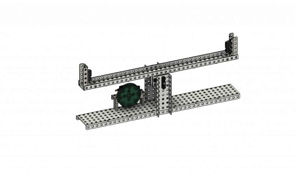
Figure 1: CAD Design of the PID Ball Balancing Seesaw.Creating the design allowed flexibility in the position of each piece and a visual reference during construction.
While the construction of the project was designed using Fusion 360, the circuit diagram of the ball balancing system was created using Fritzing.
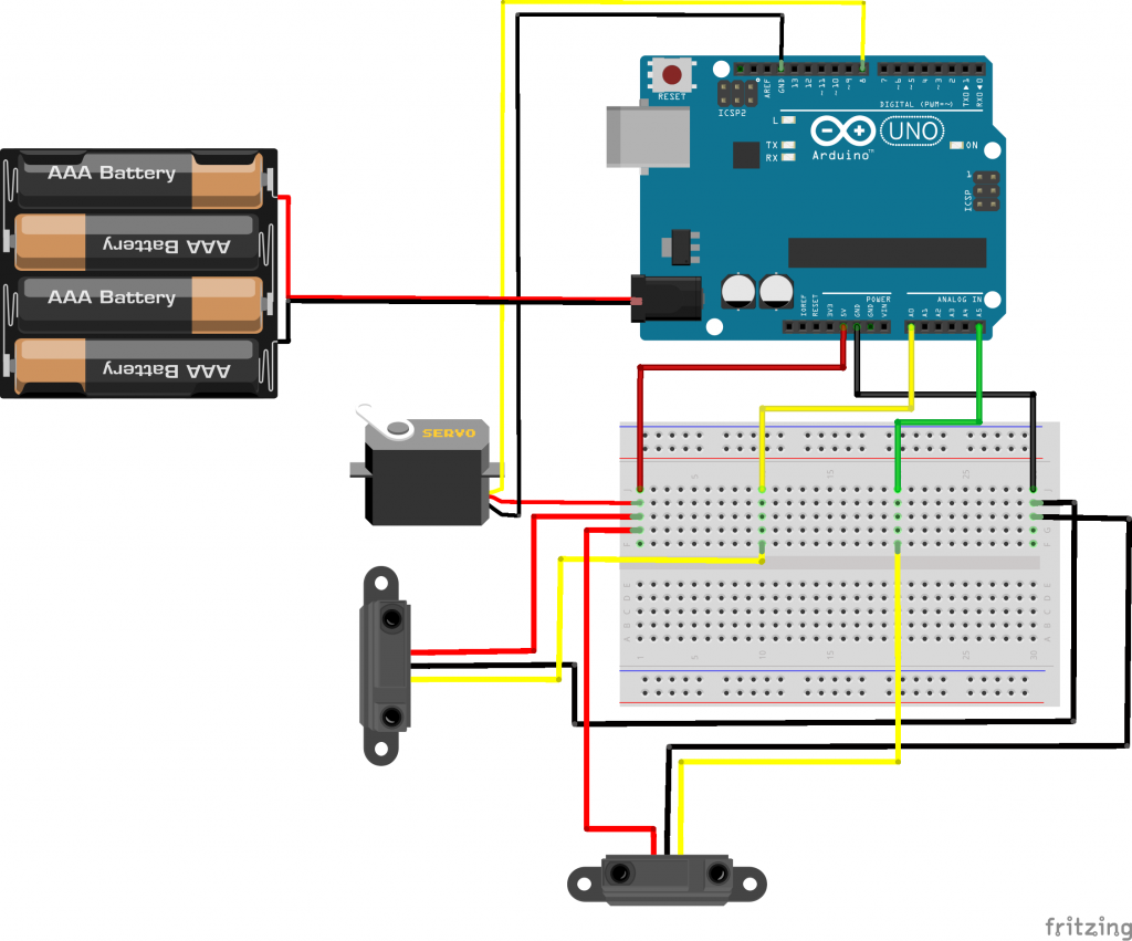
Figure 2: Circuit Diagram of the Ball Balancing System.The design helped with circuit planning and the wiring of the complete system.
The electrical component of the project consisted of two infrared distance sensors (A5 Sharp), one servomotor (Futaba), Arduino, and a 9V battery pack powering the system. The infrared distance sensor was used to determine the error between the target and the sensor value. By averaging the two sensors’ values,a precise measurement of the ball’s position can be found. To increase the accuracy of the sensors, an equation was created by curve fitting the relationship of analog reading values to centimetres
.𝑦=𝑒−((𝑥−871)/139)
x = Analog Reading Values | y = Distance in Centimetres
Equation 1: The equation used to convert analog reading values to distance in centimetres
This equation helped mitigate any big errors in the sensors’ values and allowed more precise output.
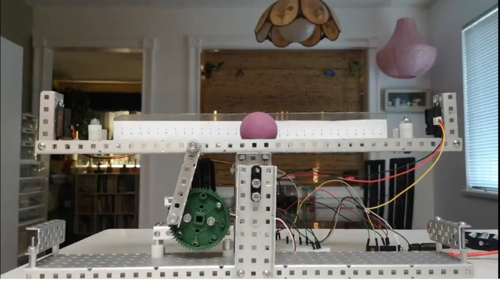
Figure 3: Wired and fully constructed PID Ball Balancing Seesaw
The parts used to create the Seesaw consisted of multiple aluminum C-Channel, standoffs, axles, and aplastic gear kit from the VEX Program. The seesaw measures approximately 2.5’’ wide by 17.5’’ long
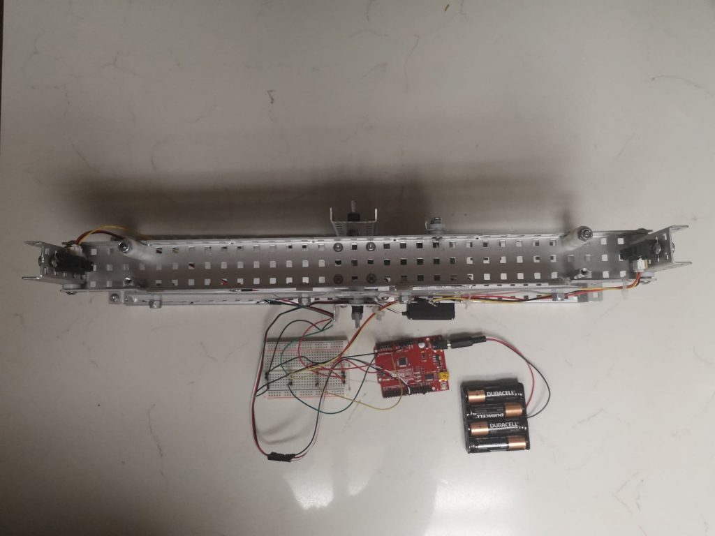
Figure 4: Top view of the PID Ball Balancing Seesaw
Software
The software used to program the system was the Arduino application in C++. A standard PID Controller was imported using the PID Library provided by Arduino. Furthermore, the results were exported from the Arduino code and imported to Google Sheets. From there, each point consisted of the time and the displacement from the center of the seesaw.All the points were then transferred and plotted on the Venier Graphical Analysis application. The software helped with analyzing trends and the global maximums or peak overshoot.
Method
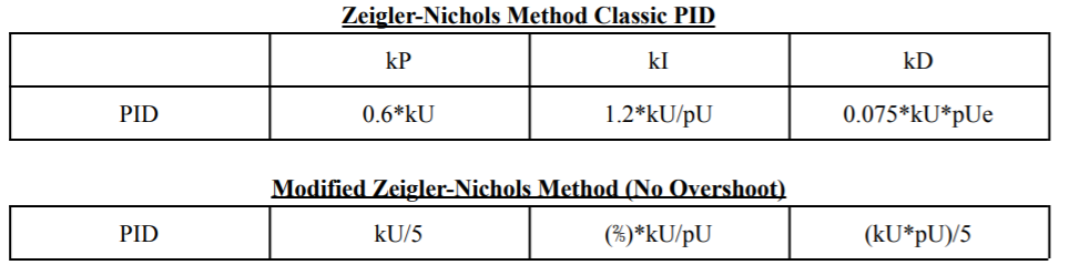
Each tuning method consisted their own distinct PID constants and was calculated using different methods. Trial and Error Method.By setting all three constants (kP, kI, kD) to zero, the PID controller is disabled and the system won’t move. To calibrate the proportional value, increase kP until the system is able to quickly move the ball to the center. Next, increase the kD in which allows the seesaw to maintain the fast motion from the kP component while minimizing any exaggerate overshoot. Last but not least, the kI value is added to mitigate any error when the system is finished and thinks the ball is in the center. Zeigler-Nichols Method.The ZN-Method sets all three constants (kP, kI, kD) to zero in the beginning,disabling the system. To start off, increase kP until there are steady continuous oscillations. The value of kP will be defined as kU. Next, by measuring the time it takes to do a full cycle from a point back to itself. The period of the oscillations will be recorded as pU. Using the table below, the PID constants can be determined.During every trial for each tuning method, the ball was placed in the same location 25 cm left from the center. The method will be compared under the three factors of peak overshoot, peak time, and settling time.
Table 1: The calculations behind the Modified and Standard Ziegler-Nichols Method.
Results
In this research, the PID constants (kP, kI, kD) have been determined using their individual methods. The obtained parameters are given in Table 2.
Table 2: PID Constants of different tuning methods
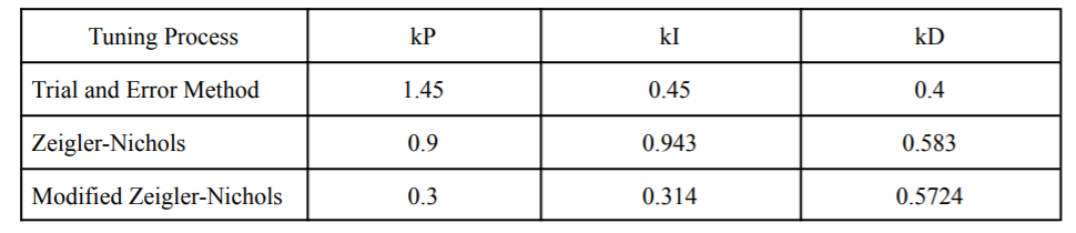
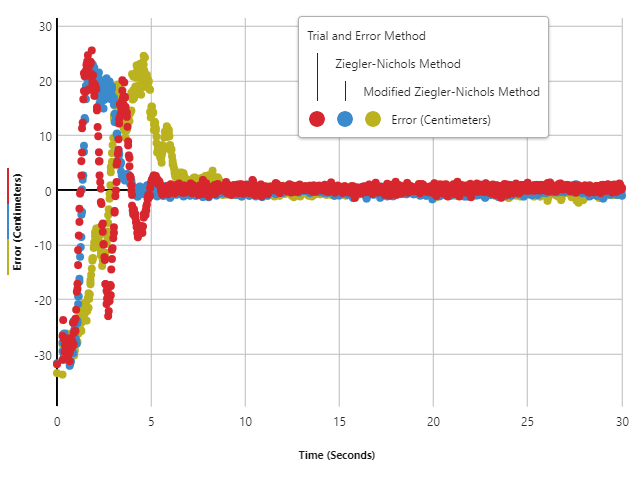
Figure 5: The displacement in the position of the ball from the center point. Points were recorded using the Arduino Program.
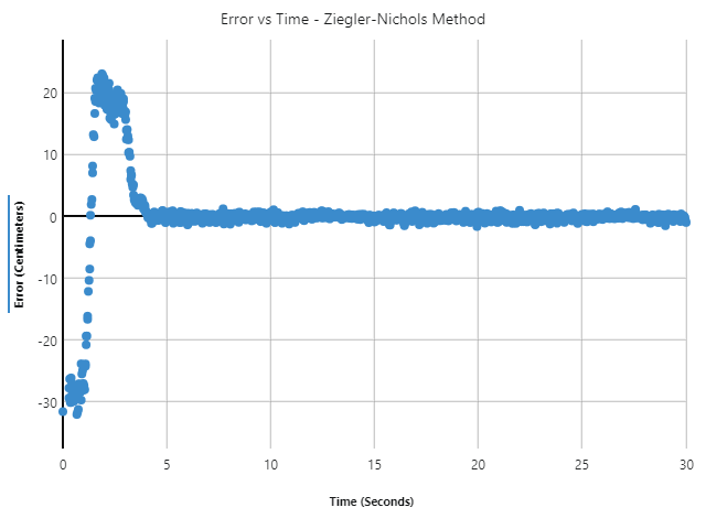
Figure 6: The displacement in the position of the ball from the center point using the Ziegler Nichols Tuning Method
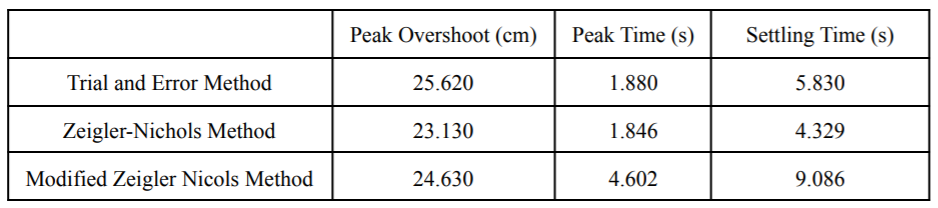
By plotting the error of the ball’s position under different tuning methods in Figure 5, it can be observed that the Ziegler-Nichols Method has the highest performance compared to the other two methods. In table3, the Zigler-Nichols Method had a lower peak overshoot,peak time, but most importantly the lowest settling time of 4.329 seconds. From Figure 6., the graph displays a gradual change in the ball’s position and very few oscillations.
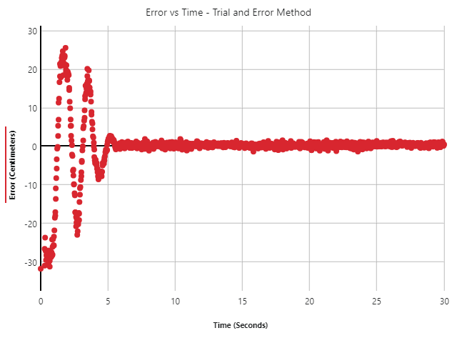
Figure 7: The displacement in the position of the ball from the center point using the Ziegler Nichols Tuning Method
While the Trial and Error Method presented a more stable solution with consistent movements, the sum of the ball’s displacement was high. This indicated a slow response time from the controller and an increase in oscillations. The huge displacement and oscillations can be seen in Figure 7 during the initial rise
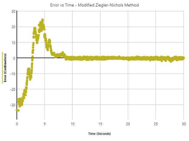
Figure 8: The displacement in the position of the ball from the center point using the Modified Ziegler-Nichols Method
Lastly, the Modified Ziegler-Nichols Method performed the worst out of all three methods. It took two times the time for the ball to reach the center relative to the other tuning methods and oscillated the most throughout the trial.
Table 3: The Comparison of different PID controllers tuning methods
Discussion
It was determined that the Ziegler-Nichols Method resulted in the lowest peak overshoot, peak time, and settling time. In a balancing system, the Zeigler-Nichols Method performed the best due to the speed and time it took for the ball to reach the center. With systems like liquid control or high precision,the application of the Ziegler-Nichols Method might not be adequate as speed is not the focus. In micro and nanometrology that use a well-controlled position stage for small components, a PID controller was tuned using different methods (Sen, 2014). However,other methods were chosen over the Ziegler-Nichols method since precision is valued. Other methods enhanced the performance of the precision position stage and decreasing the number of position errors. On the other hand, in our balancing system, speed was one of the most critical factors. However, some limitations should be noted. Due to the inconsistency of the Sharp IR Distance sensors, there were a lot of difficulties when determining the position of the ball. Although having two sensors and a conversion equation helped improve the accuracy,precise positioning specifically in millimetres was not possible. Second, only three tuning methods were chosen for this project due to the time available and the transition from in-person to virtual.In this work, different tuning methods and their performance was analyzed on a balancing system. Inconclusion, the Zeigler-Nichols Method was chosen as the best performing algorithm due to the speed it took for the ball to reach the center. Overall, the method outperformed the speed component and smoothness of the movement compared to its competition.While this paper indicates a clear performance discrepancy between all three tuning methods, other applications of these methods may have different results due to the change in the environment. However,all three tuning methods are applicable to tune a PID controller. Nonetheless, the Ziegler Method proves to have a greater performance over the manual tuning method, saving time and human labour.
References
“Common Industrial Applications of PID Control.”ControlStation, 28 Feb. 2020,controlstation.com/blog/pid-control/.
Electronoob, director.PID Balance+Ball | Full Explanation& Tuning.YouTube, YouTube, 14 July 2019,www.youtube.com/watch?v=JFTJ2SS4xyA.
Gillard, George. “An Introduction to PID Controllers.” 2017, pp. 1–16.
Krishnan, Karthik, and G. Karpagam. “Comparison ofPID Controller Tuning Techniques for a FOPDTSystem.” International Journal of Current Engineeringand Technology, 2013.
McMillan, Gregory K. “14 Industrial Applications ofPID Control .”PID Autotuning (Temperature) VI,www.physik.uzh.ch/local/teaching/SPI301/LV-2015-Help/lvpid.chm/pid_autotuning_temperature.html.“PID Theory Explained.”National Instruments, 17 Mar.2017,www.ni.com/en-ca/innovations/white-papers/06/pid-theory-explained.html.Sen,
Rajat, et al. “Comparison Between Three TuningMethods of PID Control for High PrecisionPositioning Stage.”MAPAN, vol. 30, no. 1, 2014, pp.65–70., doi:10.1007/s12647-014-0123-z.
Taip, Farah Saleena, and Ming T Tham. “Validity ofSeveral Tuning Methods for Different PIDAlgorithms.”International Journal of Engineeringand Technology, Vol. 4, no. No. 1, 2007, pp. 22–30.